CS 348 Introduction to Database Management

Introduction to databases
The relational model
Introduction to SQL
Applications and SQL
Entity relationship model
ER to RDB mapping
Normal Forms and Dependencies
Query and Update Evaluation
Concurrent Access to Data and Durability
Database Tuning

Introduction to databases

database: large and persistent collection of factual data and metadata organized to facilitate efficient retrieval and revision

data model: determines the nature of the metadata and how retrieval and revision is expressed

database management system (DBMS): program (or set of programs) that implements a data model

schema: collection of metadata conforming to an underlying data model

database instance: collection of factual data as defined by a given database schema

Three level schema architecture

external schema (view): what application programs and user see

conceptual schema: description of logical structure of all data in database

physical schema: description of physical aspects (files, devices, storage algorithms, etc)

Data independence

Idea: Applications do not access data directly but, rather through an abstract data model provided by the DBMS

physical data independence: applications immune to changes in storage structures

logical data independence: modularity

ex. the WAREHOUSE table is not accessed by payroll app; EMPLOYEE table is not accessed by inventory control app

Transaction

When multiple applications access the same data, undesirable results occur.

transaction: an application-specified atomic and durable unit of work

ACID properties:

atomic: a transaction occurs entirely, or not at all
consistency: each transaction preserves the consistency of the database
isolated: concurrent transactions do not interfere with each other
durable: once completed, a transaction’s changes are permanent

DBMS interface

data definition language (DDL): for specifying schemas

data manipulation language (DML): for specifying retrieval and revision requests

navigational: procedural
non-navigational: declarative

Summary

DBMS helps:

to remove common code from applications
to provide uniform access to data
to guarantee data integrity
to manage concurrent access
to protect against system failure
to set access policies for data

The relational model

Set comprehension for questions:

\[\{(x_1, ..., x_k) | \langle condition \rangle\}\]

Answers: all k-tuples of values that satisfy \(\langle condition \rangle\)

Relational database components

universe: a set of values \(\textbf{D}\) with equality (\(=\)) defined

relation: predicate name \(R\), and arity \(k\) of \(R\) (# of columns)

instance: a relation \(\textbf{R} \subseteq \textbf{D}^k\)

database: signature: finite set \(\rho\) of predicate names

instance: a relation \(\textbf{R}_i\) for each \(R_i\)

signature: \(\rho = (R_1, ..., R_n)\)

instance: \(\textbf{DB} = (\textbf{D}, =, \textbf{R}_1, ..., \textbf{R}_n)\)

Simple truth

Relationships between objects (tuples) that are present in an instance are true, relationships absent are false

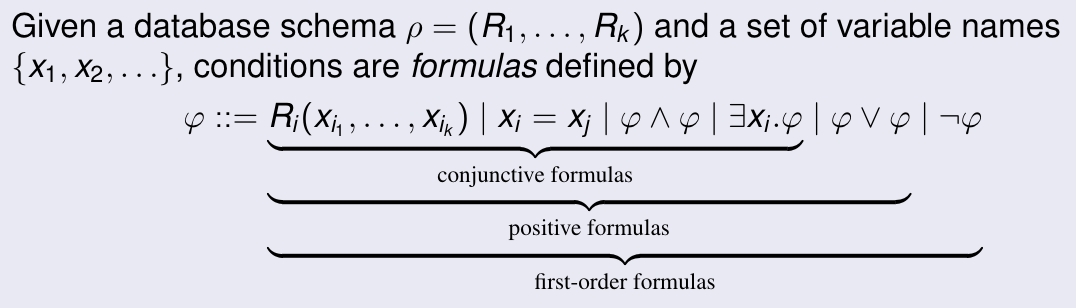
Conditions in relational calculus

Integrity constraints

yes/no conditions that must be true in every valid database instance

Domain independent query

domain independent query: a query \(\{(x_1, ..., x_k) \vert \phi\}\) such that

\[\textbf{DB}_1, \theta \models \phi \iff \textbf{DB}_2, \theta \models \phi\]

for any pair of database instances and for all \(\theta\)

Range restricted query

range restricted formula: a formula \(\phi\) such that for \(\phi_i\) that are also range restricted, \(\phi\) has the form

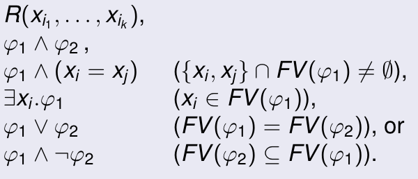
Theorem: range restricted \(\implies\) domain independent

Theorem: every domain independent query can be written equivalently as a range restricted query

What cannot be expressed in relational calculus?

RC is not turing complete

It cannot express:

built in operations (ordering, arithmetic, string operations, etc)
counting/aggregation (cardinality of sets)
reachability/connectivity (paths in a graph)

Introduction to SQL

TODO

Applications and SQL

TODO

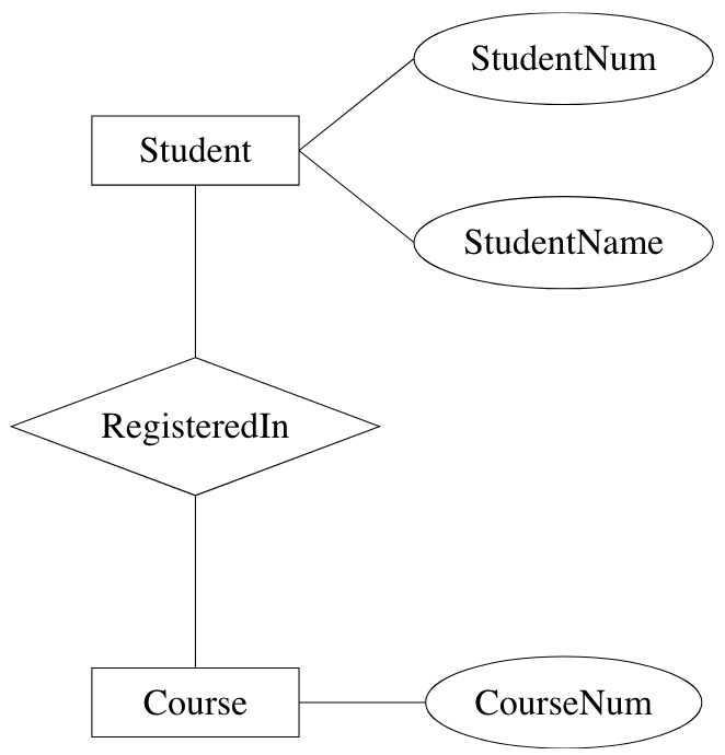
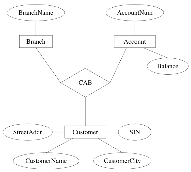
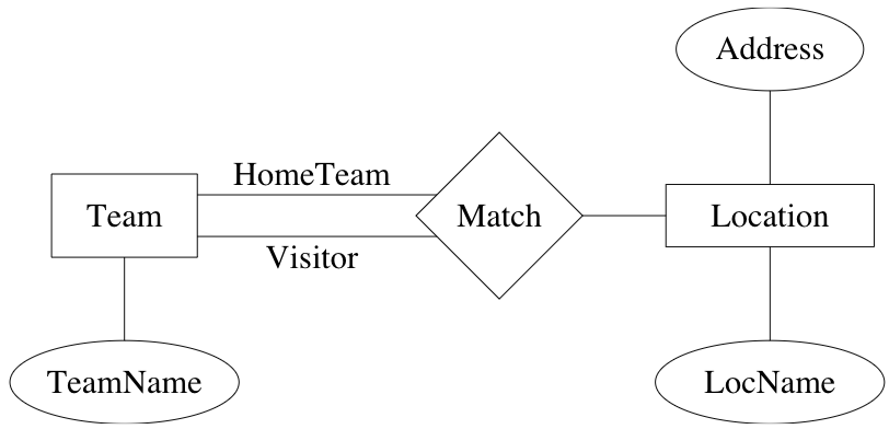
Entity relationship model

ER model

World described in terms of

entities: distinguishable object
attributes: describe properties of entities or relationships
relationships: represent certain entities are related to eachother

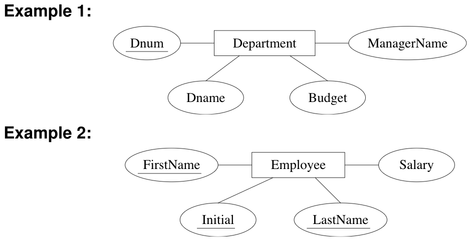
Examples:

role: function of an entity set in a relationship set

required when entity set has multiple functions in a relationship set

primary key: selection of attributes whose values determine a particular entity

many-to-many (n:n): entity in one set related to many entities in other set, and vice versa (default)

many-to-one (n:1), one-to-many (1:n): entity in one set can be related to at most one entity in the other

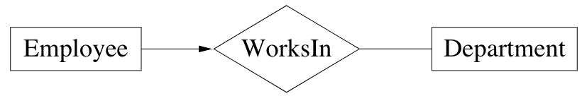
one-to-one (1:1): obvious

existence dependency: if x is existence dependent on y, then

y is a dominant entity
x is a subordinate entity

weak entity set: entity set containing subordinate entities

must have a n:1 relationship to a distinct entity set

strong entity set: entity set containing no subordinate entities

Example: transactions are existence dependent on accounts. All transactions for a given account have a unique transaction number

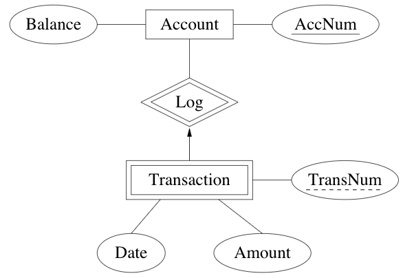
discriminator of a weak entity set: set of attributes that distinguish subordinate entities of the set, for a particular dominant entity

primary key for a weak entity set: discriminator + primary key of entity set for dominant entities

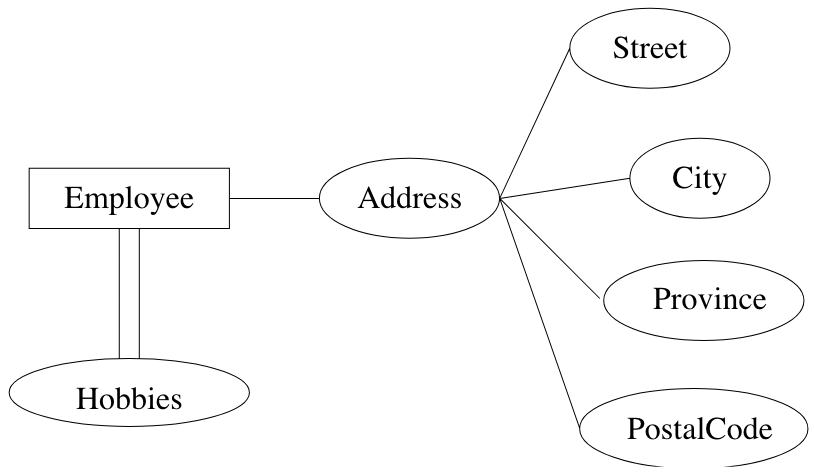
Extensions to E-R modeling

structured attributes

composite attributes: composed of fixed # of other attributes
multi-valued attributes: attributes that are set-valued

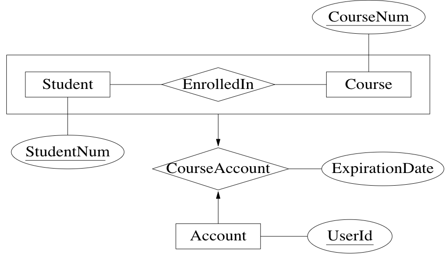
aggregation: view relationship as higher level entity

Example: accounts are assigned to a given student enrollment

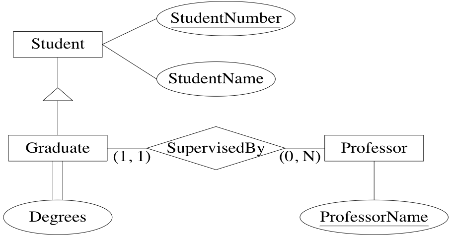
specialization: specialized kind of entity set may be derived from a given entity set

Example: grad students are students who have a supervisor and a # of degrees

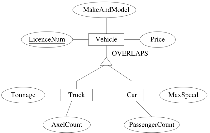
generalization: several entity sets can be abstracted by a more general entity set

Example: vehicle abstracts the notion of a car and a truck

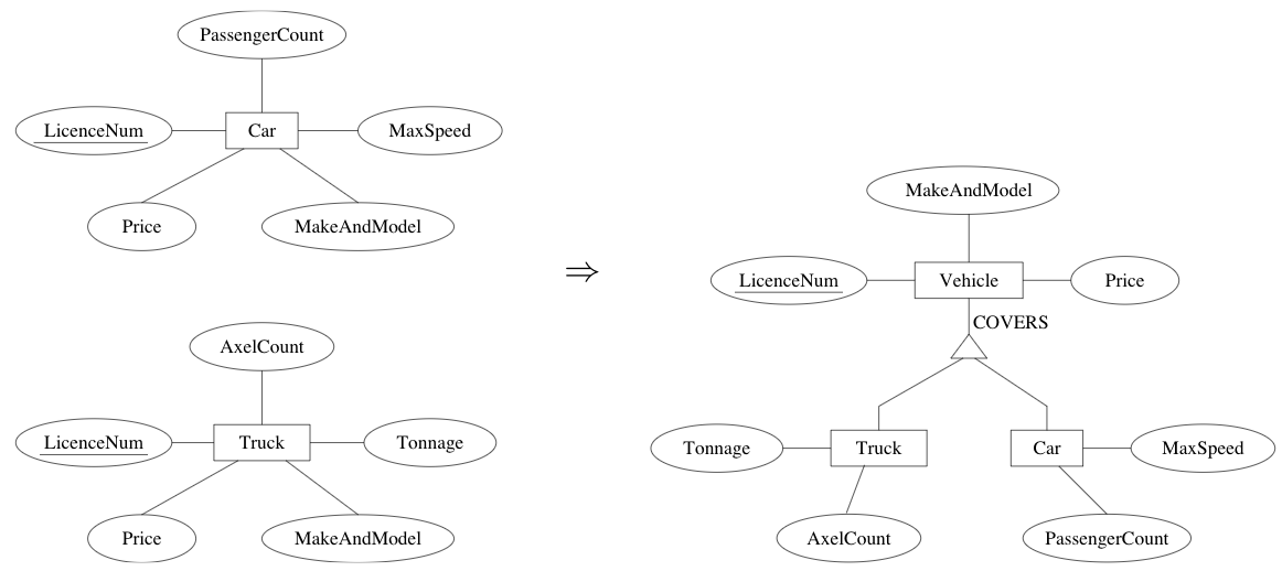
disjointness: specialized entity sets are usually disjoint but can be declared to have entities in common

Example: to accommodate utility vehicles, they can be both a car and truck via OVERLAPS

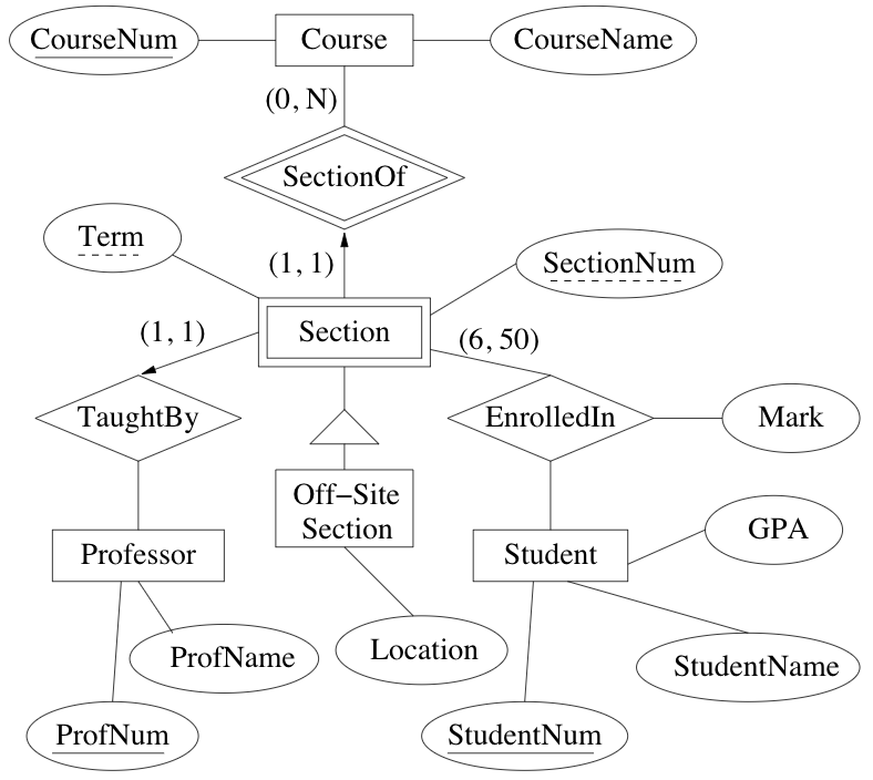
Exampe: registrar database

END OF MIDTERM CONTENT

ER to RDB mapping

Normal Forms and Dependencies

Anomalies

Problems that occur in poorly planned, un-normalized databases where all data is stored in one table.

insertion anomaly: impossible to add a piece of data without adding a related piece of data

ex. library db cannot create a new member until he/she takes out a book

deletion anomaly: a piece of data may be validly deleted, causing the unintentional deletion of another piece of related data

ex. deleting the last loan of a book may delete all information about the book from the database

Functional Dependencies

Expresses the fact that in a relational schema, the values of a set of attributes uniquely determines the values of another set of attributes.

Notation: \(X \rightarrow Y\) means \(X\) functionally determines \(Y\)

Example:

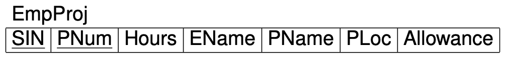
SIN \(\rightarrow\) EName
PNum \(\rightarrow\) PName, PLoc
PLoc, Hours \(\rightarrow\) Allowance

Implication for FDs

A set \(F\) logically implies a FD \(X \rightarrow Y\) if \(X \rightarrow Y\) holds in all instances of \(R\) that satisfy \(F\).

Closure \(F^+\) of \(F\) is the set of all FDs that are logically implied by \(F\).

then \(F \subseteq F^+\)

Example: If \(F = \{A \rightarrow B, B \rightarrow C\}\), then \(F^+ = \{A \rightarrow B, B \rightarrow C, A \rightarrow C\}\)

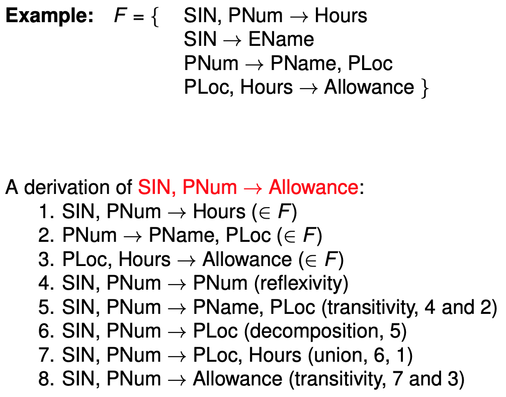
Armstrong’s axioms

reflexivity: \(Y \subseteq X \implies X \rightarrow Y\)

augmentation: \(X \rightarrow Y \implies XZ \rightarrow YZ\)

transitivity: \(X \rightarrow Y, Y \rightarrow Z \implies X \rightarrow Z\)

These axioms are

sound: anything derived from \(F\) is in \(F^+\) (ie. anything you can prove is correct)
complete: anything in \(F^+\) can be derived (ie. anything that is correct can be proved)

Additional derived rules:

union: \(X \rightarrow Y, X \rightarrow Z \implies X \rightarrow YZ\)

decomposition: \(X \rightarrow YZ \implies X \rightarrow Y\)

Example:

Keys

\(K \subseteq R\) is a superkey for relation schema \(R\) if dependency \(K \rightarrow R\) holds on \(R\)

\(K \subseteq R\) is a candidate key for relation schema \(R\) if \(K\) is a superkey and no subset of \(K\) is a superkey

primary key: a chosen candidate key

Decompositions

The collection \(\{R_1,...,R_n\}\) of relation schemas is a decomposition of relation schema \(R\) (= set of attribute) if

\[R = R_1 \cup ... \cup R_n\]

Good decompositions

do not lose information
do not complicate checking of constraints
do not contain anomalies

Lossless-Join Decompositions

A decomposition \(\{R_1, R_2\}\) of \(R\) is lossless iff the common attributes of \(R_1\) and \(R_2\) form a superkey for either schema, that is

\[R_1 \cap R_2 \rightarrow R_1 \vee R_1 \cap R_2 \rightarrow R_2\]

In other words, re-joining the decomposition always produces the exact same tuples as in the original relation \(R\).

Example:

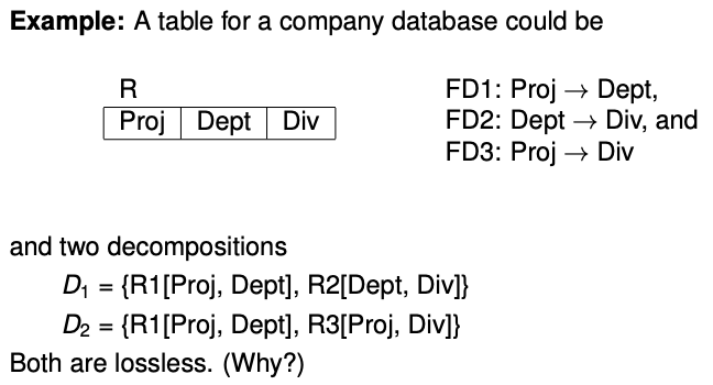
\(R_1 \cap R_2\) (= Dept) is a superkey of \(R_2\)
\(R_1 \cap R_2\) (= Proj) is a superkey of both \(R_1\) and \(R_3\)
decomposition \(D_1\) is better because FD1 and FD2 can be tested on the two separate tables. FD3 then follows from transitivity. FD2 is an interrelational constraint in decomposition \(D_2\) because testing it requires joining tables \(R_1\) and \(R_3\)

A decomposition \(D = \{R_1, ..., R_n\}\) is dependency preserving if there is an equivalent set \(F'\) of FDs, none of which is interrelational in \(D\).

Normal forms

Boyce-Codd Normal Form (BCNF)

Schema \(R\) is in BCNF w.r.t. \(F\) iff whenever \(X \rightarrow Y \in F^+\) and \(XY \subseteq R\) then either

\(X \rightarrow Y\) is trivial (ie. \(Y \subseteq X\)), or
\(X\) is a superkey of \(R\)

Formalizes the goal that independent relationships are stored in separate tables.

Third Normal Form (3NF)

Schema \(R\) is in 3NF w.r.t. \(F\) iff whenever \(X \rightarrow Y \in F^+\) and \(XY \subseteq R\) then either

\(X \rightarrow Y\) is trivial (ie. \(Y \subseteq X\)), or
\(X\) is a superkey of \(R\), or
each attribute of \(Y\) contained in a candidate key of \(R\)

First Normal Form

All data in cells is atomic.

Query and Update Evaluation

How are queries executed?

parsing, typechecking, etc
relational calculus (SQL) translated to relational algebra
optimization: efficient query plan, statistics collected about stored data
plan execution: access methods access relations, physical relational operators combine relations

Relational Algebra

Constants:

\(R_i\) one for each relational scheme

Unary operators:

\(\sigma_\varphi\) selection (filter tuples satisfying \(\varphi\), WHERE)
\(\pi_V\) projection (keep attributes in \(V\), like SELECT)

Binary operators:

\(\times\) Cartesian product
\(\cup\) union
\(-\) set difference

Theorem: for every domain independent relational calculus query there is an equivalent relational algebra expression

Iterator Model

Avoid storing intermediate results by using cursor OPEN/FETCH/CLOSE interface.

Each implementation of a relational algebra operator:

implements the cursor interface to produce answers
uses the same interface to get answers from its children

Implementations

selection: check filter condition on fetch of child
projection: eliminate unwanted attributes from each tuple
product: simple nested loops, followed by dedup
union: simple concatenation, followed by dedup
set difference: nested loops checking for tuples on r.h.s.

Naive implementations are slow, speed up using:

data structures for efficient searching (indexing)
better algorithms based on sorting/hashing
rewrite RA expr

When index \(R_{index}(x)\) is available, we replace a subquery \(\sigma_{x=c}(R)\) with accessing \(R_{index}(x)\) directly.

Even if index is available, scanning entire relation may be faster if:

relation is very small
relation is large, but most of the tuples are expected to satisfy the selection criterion

Plans

Generate all physical plans equivalent to the query, and pick the one with the lowest cost.

Simple cost model for disk I/O:

uniformity: all possible values of an attribute are equally likely to appear in a relation
independence: likelihood an attribute has a particular value in a tuple does not depend on values of other attributes

For a stored relation \(R\) and attribute \(A\) we keep the following to estimate the cost of physical plans:

\(\mid R \mid\): cardinality of \(R\)
\(b(R)\): blocking factor of \(R\)
\(\min(R,A)\): minimum value for \(A\) in \(R\)
\(\max(R,A)\): maximum value for \(A\) in \(R\)
\(\text{distinct}(R,A)\): number of distinct values of \(A\)

Cost of specific operations…

Plan generation…

Concurrent Access to Data and Durability

ACID requirements

DB implementation has two parts:

concurrency control: guarantees consistency and isolation
recovery management: guarantees atomicity and durability

Notation

\(r_i[x]\): transaction \(T_i\) reads object \(x\)

\(w_i[x]\): transaction \(T_i\) writes object \(x\)

Transaction \(T_i\) is a sequence of operations: \(T_i = r_i[x_1], r_i[x_2], w[x_1], c_i\)

\(c_i\): commit request of \(T_i\)

For a set of transactions \(T_1, ..., T_k\), we want to produce a schedule \(S\) of operations such that

every operation \(o_i \in T_i\) also appears in \(S\)
\(T_i\)’s operations in \(S\) are ordered as they are in \(T_i\)

Serializability

Goal: produce a correct schedule with maximal parallelism

correctness: must appear as if the transactions have been executed sequentially

An execution of \(S\) is serializable if it is equivalent to a serial execution of the same transactions.

Example:

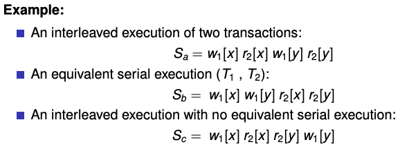
recoverable schedule: no operations are non-recoverable

cascadeless schedule (ACA): does not have cascading abort

if \(w_i[x], ..., r_j[x]\) then must also have \(c_i, ..., c_j\)
every cascadeless schedule is also recoverable

For every operation that a scheduler receives from a query processor, it can:

execute it: send to lower module
delay it: insert to queue
reject it: cause abort of transaction
ignore it: no effect

conservative scheduler: favours delaying operations

aggressive scheduler: favours rejecting operations

Two Phase Locking (2PL)

Transactions must have a lock on objects before access

shared lock for reading an object
exclusive lock for writing an object

2PL protocol: transaction has to acquire all locks before it releases any of them

Theorem: 2PL guarantees the produced transaction schedules are (conflict) serializable

STRICT 2PL: locks held until commit, avoids cascading aborts (ACA)

Isolation Levels in SQL

4 isolation levels:

level 3 (serializability): table-level strict 2PL
level 2 (repeatable read): tuple-level strict 2PL
- phantom tuple may occur (results from insert/delete during “all records” query)
level 1 (cursor stability): tuple-level exclusive-lock only strict 2PL
- reading same object twice may result in different values
level 0: neither read nor write locks are required, transaction may read uncommitted updates

Recovery

Goals:

allow transactions to be
- committed: with a guarantee that the effects are permanent, or
- aborted: with a guarantee that the effects disappear
allow the database to be recovered to a consistent state in case of HW failure

Approaches to recovery:

shadowing
- copy-on-write and merge-on-commit
- poor clustering
- not used in modern systems
logging
- use of log (separate disk) to avoid forced writes
- utilization of buffers
- preserves original clusters

Log Based Approaches

Logs are read/append only, and transactions add log records about what they do.

Types of information:

UNDO: old versions of modified objects, used to undo changes made by a transaction which aborts
REDO: new versions of modified objects, used to redo changes made by a transaction which commits
BEGIN/COMMIT/ABORT: recorded whenever a transaction changes into one of these states

Log example:

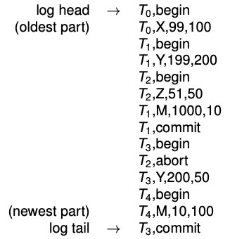
To ensure the log is consistent with main database, use write ahead log (WAL). Requires:

UNDO rule: a log record for an update is written to log disk before the corresponding data is written to the main disk
- guarantees atomicity
REDO rule: all log records for a transaction are written to log disk before commit
- guarantees durability

Database Tuning

physical design: process of selecting physical schema (data structures) to implement a conceptual schema

tuning: periodically adjusting physical or conceptual schema to adapt to requirements via:

making queries run faster
making updates run faster
minimizing congestion due to concurrency

Both of the above rely on understanding the workload.

workload description includes:

most important queries/updates and their frequency
desired performance goal for each query/update
include the relations/attributes accessed/retrieved, selectiveness of join conditions

Physical Schema

Storage strategy for each relation. Possible options:

unsorted (heap) file
sorted file
hash file

Add indexes which:

speed up queries
increase update overhead

Indexes

Create/drop syntax:

CREATE INDEX LastnameIndex
ON Employee(Lastname) [CLUSTER]

DROP INDEX LastnameIndex

Effects of index:

reduce execution time for selections with conditions involving Lastname
increase insertion execution time
increase or decrease execution time for updates or deletions of rows
increase amount of space required to represent Employee

An index on attribute \(A\) of a relation is clustering if tuples with similar values for \(A\) are stored together in the same block.

Other indices are non-clustering.

A relation has at most one clustering index.

Two relations are co-clustered if their tuples are interleaved within the same file.

useful for hierarchical data (1:n relationship)
can speed up joins (particularly foreign key join)
sequential scans of either relation slow down

Creating multi-attribute index:

CREATE INDEX NameIndex
ON Employee(Lastname, Firstname)

tuples are organized first by Lastname, then Firstname

useful for:

SELECT *
FROM Employee
WHERE Lastname = 'Smith'

SELECT *
FROM Employee
WHERE Lastname = 'Smith'
AND Firstname = 'John'

extremely useful for:

SELECT Firstname
FROM Employee
WHERE Lastname = 'Smith'

SELECT Firstname, Lastname
FROM Employee

not useful at all for

SELECT *
FROM Employee
WHERE Firstname = 'John'

Tuning the Conceptual Schema

Unlike physical schema changes, conceptual schema changes often can’t be completely masked from end users.

normalization: process of decomposing schemas to reduce redundancy

denormalization: process of merging schemas to intentionally increase redundancy

Generally redundancy increases update overhead due to change anomalies, but decreases query overhead (due to less joins?).

partitioning: of a table means to split it into multiple tables to reduce bottlenecks

horizontal: each partition has all the original columns and a subset of original rows
- separates operational from archival data
vertical: each partition has a subset of original columns and all the original rows
- separates frequently used columns from eachother or from infrequently used columns

Tuning Queries

Physical and conceptual schema changes impact all queries.

Guidelines:

sorting (ORDER BY, DISTINCT, GROUP BY) is expensive
when possible, replace subqueries with joins
when possible, replace correlated subqueries with uncorrelated subqueries
use vendor tools to examine query execution plan

Tuning Applications

Guidelines:

minimize communication costs
- return fewest columns and rows necessary
- update multiple rows with WHERE rather than a cursor
minimize lock contention and hot spots
- delay updates and operations on hot spots as long as possible
- shorten/split transactions as much as possible
- perform insert/update/delete in batches
- consider lower isolation levels

Contents

Introduction to databases

Three level schema architecture

Data independence

Transaction

DBMS interface

Summary

The relational model

Relational database components

Simple truth

Conditions in relational calculus

Integrity constraints

Domain independent query

Range restricted query

What cannot be expressed in relational calculus?

Introduction to SQL

Applications and SQL

Entity relationship model

Extensions to E-R modeling

Exampe: registrar database

END OF MIDTERM CONTENT

ER to RDB mapping

Normal Forms and Dependencies

Anomalies

Functional Dependencies

Implication for FDs

Armstrong’s axioms

Keys

Decompositions

Lossless-Join Decompositions

Normal forms

Boyce-Codd Normal Form (BCNF)

Third Normal Form (3NF)

First Normal Form

Query and Update Evaluation

Relational Algebra

Iterator Model

Plans

Concurrent Access to Data and Durability

Notation

Serializability

Two Phase Locking (2PL)

Isolation Levels in SQL

Recovery

Log Based Approaches

Database Tuning

Physical Schema

Indexes

Tuning the Conceptual Schema

Tuning Queries

Tuning Applications